practice

• age: defendant’s age

• c_charge_degree: degree charged (Misdemeanor of Felony)

• race: defendant’s race

• age_cat: defendant’s age quantized in “less than 25”, “25-45”, or “over 45”

• score_text: COMPAS score: ‘low’(1 to 5), ‘medium’ (5 to 7), and ‘high’ (8 to 10).

• sex: defendant’s gender

• priors_count: number of prior charges

• days_b_screening_arrest: number of days between charge date and arrest where defendant was screened for compas score

• decile_score: COMPAS score from 1 to 10 (low risk to high risk)

• is_recid: if the defendant recidivized

• two_year_recid: if the defendant within two years

• c_jail_in: date defendant was imprisoned

• c_jail_out: date defendant was released from jail

• length_of_stay: length of jail stay

import numpy as np
import pandas as pd
import scipy
import matplotlib.pyplot as plt
import seaborn as sns
import itertools
from sklearn.metrics import roc_curve
import warnings
warnings.filterwarnings('ignore')

clean_data_url = 'https://raw.githubusercontent.com/ml4sts/outreach-compas/main/data/compas_c.csv'

df= pd.read_csv(clean_data_url,
                 header= 0).set_index('id')

df.head()

	age	c_charge_degree	race	age_cat	score_text	sex	priors_count	days_b_screening_arrest	decile_score	is_recid	two_year_recid	c_jail_in	c_jail_out	length_of_stay
id
3	34	F	African-American	25 - 45	Low	Male	0	-1.0	3	1	1	2013-01-26 03:45:27	2013-02-05 05:36:53	10
4	24	F	African-American	Less than 25	Low	Male	4	-1.0	4	1	1	2013-04-13 04:58:34	2013-04-14 07:02:04	1
8	41	F	Caucasian	25 - 45	Medium	Male	14	-1.0	6	1	1	2014-02-18 05:08:24	2014-02-24 12:18:30	6
10	39	M	Caucasian	25 - 45	Low	Female	0	-1.0	1	0	0	2014-03-15 05:35:34	2014-03-18 04:28:46	2
14	27	F	Caucasian	25 - 45	Low	Male	0	-1.0	4	0	0	2013-11-25 06:31:06	2013-11-26 08:26:57	1

df.tail()

	age	c_charge_degree	race	age_cat	score_text	sex	priors_count	days_b_screening_arrest	decile_score	is_recid	two_year_recid	c_jail_in	c_jail_out	length_of_stay
id
10994	30	M	African-American	25 - 45	Low	Male	0	-1.0	2	1	1	2014-05-09 10:01:33	2014-05-10 08:28:12	0
10995	20	F	African-American	Less than 25	High	Male	0	-1.0	9	0	0	2013-10-19 11:17:15	2013-10-20 08:13:06	0
10996	23	F	African-American	Less than 25	Medium	Male	0	-1.0	7	0	0	2013-11-22 05:18:27	2013-11-24 02:59:20	1
10997	23	F	African-American	Less than 25	Low	Male	0	-1.0	3	0	0	2014-01-31 07:13:54	2014-02-02 04:03:52	1
11000	33	M	African-American	25 - 45	Low	Female	3	-1.0	2	0	0	2014-03-08 08:06:02	2014-03-09 12:18:04	1

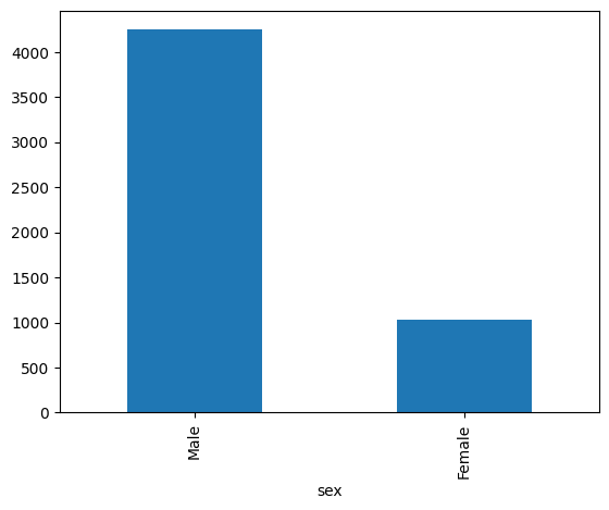
Sex = df['sex'].value_counts()

Sex.plot(kind= 'bar')

<Axes: xlabel='sex'>

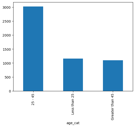
Age= df['age_cat'].value_counts()

Age.plot(kind= 'bar')

<Axes: xlabel='age_cat'>

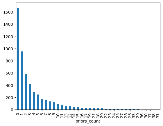
priorA= df['priors_count'].value_counts()

priorA.plot(kind= "bar")
# 0 is the most common number of prior arrest!!!

<Axes: xlabel='priors_count'>

REa= df['two_year_recid'].value_counts()

REa.plot(kind= 'bar')

<Axes: xlabel='two_year_recid'>

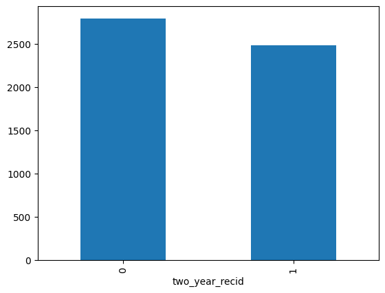
REa

two_year_recid
0    2795
1    2483
Name: count, dtype: int64

2483/(2483+2795)*100
# math to find the exact percentage

47.04433497536946

# 47% of people got re-arrested!!!

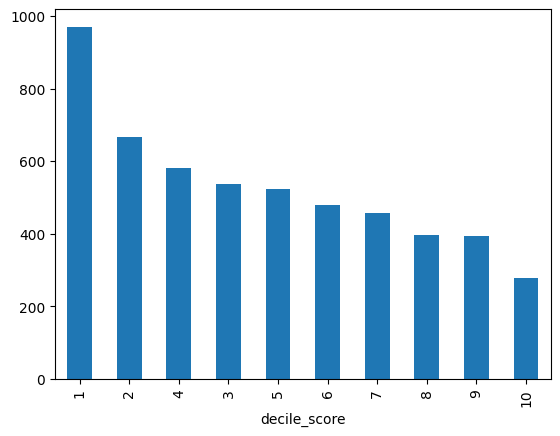
compasS= df['decile_score'].value_counts()

compasS.plot(kind= 'bar')
#  1 is the most common score!!!

<Axes: xlabel='decile_score'>